Statistical Tools
The Historical Reconstruction of Gross Domestic Product Before 1950: A Study of Statistical Tools in Practice
One of the many questions at the heart of economic history is, when did some countries become rich and how has their wealth persisted over time and space? Or, better still, what sectors of the economy have been at the center of economic growth from a historical perspective? To answer these questions effectively, it is crucial to understand how the wealth of countries evolved over time and space, the origins of such wealth, the peculiar circumstances that made such economic growth possible, and whether that economic growth persisted or changed. One way to answer these questions is by estimating GDP and GDP per capita for economies dating back to the medieval period. More recently, GDP is perhaps the most obsessed-about economic phenomenon, possessing the capacity to make or mar political administrations. Advances in historical national accounting methods mean that the estimates necessary for this assessment are now available for several European economies.
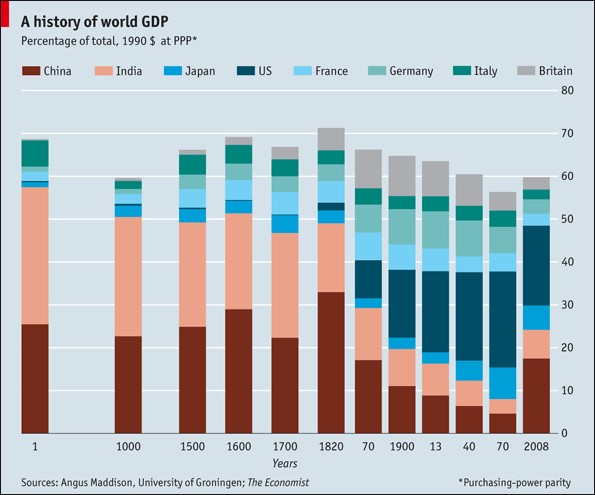
Such information also contributes to the other controversial debates. For instance, on October 14th, 2014, The Economist published a controversial global economic history chart (the above chart), illustrating progressively the share and distribution of global GDP for major world economies since 1AD. Several scholars have argued that China is reclaiming the title of the largest economy in the world. As is evident in the graph, China began as a leading economy, and her place in the world has flunctuated throughout history. For some scholars, the chart gave credibility to observations that India’s economy shrank and was depleted because of British colonization. For many others, the methodology and data behind the assertions were dubious. After all, the researcher credited with these findings, Angus Maddison, described them as "mere conjectures.”
In the light of the above, it is the goal of this essay to inform the reader of the production process (the most common sources of such data, the extrapolation techniques, benchmark estimates, and the most common assumptions guiding researchers’ estimates) behind several national estimates. By focusing on the global estimates produced by renowned researcher Angus Maddison, it is possible to reveal that “guesstimates” and extrapolations by different researchers can lead to different estimates, even if by a small margin. This point is important because it is often assumed that using either of the three assessed methods to calculate a nation’s GDP should yield the same results.
The first section begins by clarifying the relatively modern concept of GDP and traces the origins of the concept as it is understood today, highlighting the early extrapolation efforts for several advanced economies. The next section highlights the methods and sources of data employed by national accounting researchers for formulating estimates for periods earlier than 1950.
For clarity and an overview, the focus is placed on Angus Maddison. His research on global estimates provides the most comprehensive attempt to estimate global GDP from early periods. Furthermore, Maddison is particularly interesting because of the constant updates to his work via the Maddison Database Project. As the purpose of this essay is to help the reader understand how these estimates are constructed and reconstructed, a typical example is presented.
How does the Concept of Gross Domestic Product Concept Work?
Gross domestic product refers to an economy’s productive and income-generating capacity. It is the total monetary or market value of all the finished goods and services within a country’s borders in a specific year. The metrics present a sort of medical report for the economy of any country; in this case, they report the state of the world economy throughout history.
The most common approach today is the expenditure approach, combining consumption, government expenditure, savings, investments, and net exports (exports subtracted from imports). There is also the income approach, which compiles data from employment and earnings surveys to estimate salaries and wages by industrial activity. This approach often includes personal income, disposable income, proprietor’s income, corporate profits, net interest paid, and indirect taxes. Finally, there is the production approach, which includes GDP production counted by sector of activity, and tools such as the Index of Industrial Production (IIP), physical quantity indicators, and sales-type statistics for estimates of value-added in manufacturing. A major drawback of this approach is the difficulty in differentiating between intermediate and final goods. Hence, the preference of countries such as the United States (US) and Japan for the income or expenditure approaches.
Today, national statistics offices are often responsible for collating the necessary data for the above-mentioned components, depending on the method adopted by the country. However, previously, such statistical offices did not exist, and even if they did, decisions on what to measure and what not to are likely to have changed as economies involved. Nonetheless, it is this ambitious task that Angus Maddison set himself.
A Brief History of the Concept of Gross Domestic Product
The history of GDP is often traced to the development of national income accounts by Simon Kuznets7 to assess US Government efforts to address the Great Depression, but the story begins much earlier and can be periodized into three phases: the early estimates (1600–1930), a brief revolutionary period (1930–1950), and the recent era of international guidelines (1950–present)8. Each phase was dictated by a combination of national idiosyncrasies and international events.
William Petty is credited with making the first efforts to estimate national income, which became popularly known as “political arithmetic” in 1665. In 1696, Gregory King 9 employed a variety of techniques regarding income, expenditure, and production to estimate the English national income. He created broad national income accounts that revealed the distribution of annual national income, savings, and expenditure by social and occupational groups.
Throughout the 18th century, other countries also attempted to measure their economies. In 1790, Russian national income estimates were produced; in 1798, the Netherlands provided its first estimates; Germany, India, Greece, Austria, Australia, and the US followed in the 19th century. Complementing these early efforts were the publications of private institutions such as the National Industrial Conference Board and the Brookings Institution. The prevailing idea in the early national accounts of various countries was that national income depended on how much was available to spend now and how much remained for increasing the national stock of assets.
Several historical accounts of the origin of GDP begin in the revolutionary phase. However, even this era can be further divided into the interwar period, plagued largely by a global depression, and the effects of the global outbreak of the Second World War. The theoretical foundations were further shaped by the publication of Alfred Marshall’s Principles of Economics in 1890. Colin Clark was tasked by the British Government to assess national income expenditure throughout the 1930s 11. With great thoroughness, he highlighted the components of production, expenditure, and government finances, accounting for inflation and income distribution.
Across the Atlantic, in the US, Simon Kuznets submitted a report to Congress in 1934 that revealed that the national income had halved between 1929 and 1932. This report helped create a wider policy scope and was cited in the supplementary budget sent by Franklin Roosevelt to Congress. Nonetheless, there were several issues with Kuznets’ estimates. For example, he opposed the inclusion of government defense spending in the national estimates because of the likelihood of the implicit assumption that it may count towards the welfare of individuals. Milton Gilbert, Head of the US Commerce Department, believed the opposite. Therefore, Kuznets was concerned about a national estimate that estimated welfare and not just economic output. This debate remains throughout the development of a standardized national accounts system, with defense spending recently being included as part of government spending and revealing an increase in the economy even for countries in conflicts despite the possible contraction in national welfare. Ultimately, Gilbert won, and this marked a change from a mainly private perspective of the economy to include the government as a participating entity in the economy.
Contributing further to the theoretical foundations of the concept of national income and GDP was The General Theory of Employment, Interest and Money by John Maynard Keynes. He claims that savings are equal to investment and argues for a widely accepted definition of income, consumption, investment, and saving, all of which are relevant components of national income estimates today.
In the US, the decision to prioritize national accounts was as a result of the pressure from Maynard Keynes’ during the wartime period. These accounts were prepared by James Meade and Richard Stone. Consultations between the British, Canada and the US happened in 1944 to create a standard set of concepts and procedures. As Europe moved beyond the war, these national accounts served as “political necessity” to assess the needs of Marshall Aid and burden-sharing in the North Atlantic Treaty Organisation (NATO).
Richard Stone led the committee to develop a standardized approach for the Organization of European Economic Community (OEEC) for the above-stated purpose. In 1950, the OEEC system was merged with the United Nations (UN) system in most countries except for communist ones. This standardization meant that, from as early as 1950, there were and are comparable estimates for about 150 countries across the world. Often referred to as the Standard of National Accounts (SNA), this provides a coherent macroeconomic framework to allow economies to be comparable. The SNA (for example, there is the SNA 1968, SNA 1993, SNA 2008) approach is updated regularly to include new sectors in the economy. Some countries have used these account standards to extrapolate the national estimates for various countries. In the European Union (EU), all member countries must report their accounts in a standard similar to the SNA. This method is called the European System of Accounts (ESA 1970, ESA 1996, and ESA 2010). These standards make it easier for researchers to estimate GDP after 1950 much more accurately than for earlier periods.
This standardized system presents a unified macroeconomic framework to account for the entire economy, which can be crosschecked in three major ways. From the production account, the value is calculated as the sum of the value-added in the various sectors of the economy (e.g. agriculture, industry, services, net of duplication). There is also the sum of the final expenditures account, principally recording the final expenditures by consumers, investors, and government. The final account is the income account recording the total of wages, rents, and profits. These accounts, fully integrated, allow for easily describing volume, value, relative, and absolute prices and changes in economic structure.
Several European countries have data extending to as early as 1820. Most African countries have data only from 1950, with the exemption of Ghana, South Africa, and Egypt having early information from 1913. Lack of earlier data means extrapolations are nearly impossible and this can only be solved by the discovery of new information regarding national accounts or economic sectors for earlier periods. It is possible to create estimates for Asia for as early as 1900 in countries such as Thailand, Taiwan, South Korea, Bangladesh, Burma, and the Philippines. Earlier estimates are also possible for China, Indonesia, and Japan. In Latin America, it is possible to derive estimates as early as 1900, with some countries, such as Brazil, dating back as far as 1820.
While the focus of this research is on estimates before 1950, these years are distant and it would be wrong to assume that just one approach or set of approaches were adopted for most countries. Several developing countries could not boast statistical offices before 1950 (some are still reliant on the International Monetary Fund [IMF] for national estimates). Therefore, the years from around 1870 until 1950 appear rather easier regarding more accurate data; earlier periods often have inconsistent data or, sometimes, the data are simply unavailable. Some of the relevant data often include population censuses and wages paid to construction workers archived in company reports. Often, it is possible to extrapolate this information by making broad general assumptions about, for instance, daily required nutrients, based on written diaries or news reports. For countries where interpolations or extrapolation is impossible, the gaps are simply assumed by the researcher or, in the event of uncertainty, the spaces are left blank. However, this is only a last resort; there are often hints that guide researchers in international statistics books.
Measuring Gross Domestic Product in Historical Perspective: Methods and Sources
In many European countries, there is abundant quantitative information about economic estimates before 1950, especially the UK and the Netherlands. Therefore, it has been possible for scholars to create well-stocked archives. In countries with limited existing data, scholars such as Alvarez-Nogal and Prados de la Escosura (2013) have used short-cut methods. The economy is divided into agriculture and non-agriculture, with output in the agricultural sector derived through a demand function of the population, real wages, and the relative price of food. In addition, international trade is assumed to be in food. To estimate the non-agricultural sector, however, the output is assumed to have centered around urban population, accounting for both rural industry and the popular concept of “agro-towns.” This output-oriented approach bridges the gap between the macro approach of growth economists and the sectoral approach perspective of much of economic history.
For a “longer-cut” to determine national estimates, it is common for researchers to divide the economy into broader sectors: a). agricultural, b). industry or manufacturing, and c). service sectors13. Agricultural output is mainly estimated using data from the amount of cultivated land and crop yields per unit of land. Industrial output is determined by four sub-sections: food and processing, metals and mining, textiles and other manufacturing, and building. The data for metals and mining are sometimes available from several government sources as they can mainly be estimated using the volume of output of iron, copper, zinc, coal, etc. The service sector is also sub-categorized, into commerce, government, housing, and domestic sources.
Overall, there are two main ways to measure historical GDP. The first method, invented by Angus Maddison, extrapolates back from recent estimates of GDP per capita using purchasing power parity (PPP) based on constant-price indices of GDP per capita. The second benchmark method is estimating the components of the GDP in their nominal values and then adjusting for differences in international price levels. If these historical estimates were perfectly similar, they should yield the same estimates.
Another common technique is to construct a growth series, link it to a specific benchmark, and extrapolate backward to arrive at earlier income levels. Some scholars have often simply highlighted different benchmarks, as observed in the recently published Maddison Database 2018. This is usually achieved by calculating growth patterns in years for which reliable estimates are feasible and then assuming either an increasing fixed-growth percentage in the preceding years or using alternative sources, such as historical records, to predict decline or increase in the growth pattern in years for which less reliable years are available. A detailed example of this approach is presented with a pictorial example, below. Further complicating the ability to compare economies across time and regions are the different consumption patterns in premodern economies. Often, the technique adopted was to adjust different consumption baskets to caloric and protein components. Such an approach is necessary to estimate the consumption and price of goods factor of the GDP equation.
The above-described approach is often not as tedious as developing pre-war economic estimates (mostly from 1950 backward until 1870); some countries have “official or quasi-official” accounts, for example, Austria in 1830, Finland 1860, Norway 1865, the Netherlands 1900, Germany 1925, Canada 1926, and the US 1929. Except in countries where such official or quasi-official statistics were present, many government officials and scholars have followed the UN/OECD (Organisation for Economic Co-operation and Development) guidelines to link their series with post-war estimates. Many of individuals tasked with developing a system of national accounts were influenced by Simon Kuznets’ backward extrapolation of US national estimates. Other notable scholars include Charles Feinstein in the UK, Kazushi Okhawa in Japan, Noel Butlin in Australia, Olle Krantz in Sweden, Riitta Hjerpee in Finland, and Gallman and Kendrick in the US. However, many of these estimates were inconsistent and difficult to compare. For example, the estimates for New Zealand relied on proxy estimates; in Switzerland, the estimates relied on deflated income.
Addressing problems of comparability, economists and historians often adopt different techniques. For developed countries between 1850 and 1950, it is often possible to make reconstructions based on historical statistical data such as production series, wages, and employment. For less-developed countries, the choice is often more limited to import–export statistics of major products. The next section discusses the prominent sources used by economic historians in deriving economic estimates.
Despite the existence of a standard measure that can be used to extrapolate, many national accounts for these earlier periods appear problematic because statistical offices in the different countries had differing perspectives regarding what is and is not part of the economy. The UK and US used mainly income flows, many of which are from tax sources, whereas Germany produced output information from industrial surveys, and France mainly produced input–output tables.
However, there is no danger in overestimating or underestimating growth as a result of differences in measuring the economy, primarily because statistical offices often have elaborate techniques to crosscheck information by using input–output tables. However, in economies that relied on services, it is often difficult to measure the economy. Therefore, in some countries, proxy sources such as employment indicators are used.
As stated previously, there are reliable accounts for the major economies of the world from 1950, and relatively credible estimates for major economies of the world dating to 1870. However, for longer-term estimates, a set of relatively unique series of sources is adopted by researchers. It is important to understand the various ways these estimates are derived, because researchers such as Angus Maddison use this information to create a picture of global economic history in quantitative terms.
How do economists and historians obtain data to produce comparable estimates to allow for the production of national accounts for periods earlier than 1870, and what are the challenges of working with their sources?
The most common sources for many economists and historians are surviving documents from monasteries, hospitals, churches, courts, and private estates. These are often studied to provide wages, rents, and prices and to observe the distribution of wealth and track how human capital has developed throughout history. For example, Chaney and Hornbeck (2015) studied tithing records of the Archbishop of Valencia (there was a mandatory 10% tithe) to estimate agricultural productivity of Morisco-dominated regions. Production and consumption patterns can also be determined by studying Cape probate inventories (Fourie & Van Zanden, 2013). Furthermore, records from the Imperial Ministry of Justice in China containing information on agricultural wages over time were used by Allen et al. (2011) to contribute to perhaps the most popular economic history debate regarding whether incomes were higher before the Industrial Revolution. The most popular sources of information, at least by most of the referenced scholars in Maddison’s estimates, are the statistical handbooks of various regions and countries.
When the wages of a society or region are accessed, whether through statistical books or company accounts, scholars need to convert the wages from that period into real wages. The internationally comparable “subsistence basket method”16 is a practical approach for this. This basket method is controlled to include regional specifications, the consumption of luxury items, and other peculiarities. A typical barebone basket can be used to measure price fluctuations and consumption needs and methods. This method assumes that an individual requires 2100kcal per day to provide enough nutrients to survive and work. This calory requirement17 is also as stipulated by the World Bank poverty line as corresponding to $1.2518. Therefore, the method focuses on the consumption of necessities. The researcher then considers weight and height to account for the degree of differences in consumption across different countries 19.
Regarding population data, information on the evolution of the Bolivian population, for example, is scarce as there are no annual official statistics in the 19th century, but there are estimates for different benchmark years (1825, 1831, 1835, 1846, 1854, 1882).
Below is an example of a historical source. The document contains information about the population and death and birth rates in Hamburgischen Staates.
However, these sources are often fragile and based on studies that compare scattered output, consumption, and demographic data, leading to often debatable results. Working with historical sources can be complex. For instance, borders have changed immensely over time, which presents a problem for assessing the economic output or productivity of a region. The prevailing convention in economic history is to use contemporary borders; however, sometimes, this is difficult. While it is easy to acknowledge the economic strength of the Roman Empire, how do we assess the productivity of the various states that broke out of its collapse?
Dealing with sources is further complicated by the language in which they were recorded, some of which are difficult to interpret, or the units in which the data is calculated is difficult to interpret (i.e measurements styles and standards varied across countries). It is often the norm that researchers make units comparable, but even this is complex; for instance, in Scotland, each of the 20-odd shires (regions) had a unique measurement of grain called a boll (as reported in Palma, 2019).
For advanced countries before 1950, the data required to make such early estimates are readily available. The image, below, is of GDP estimates for Australia from 1788 to 1939. How these data were derived is typical of how early estimates are sourced. The prices of agricultural output are taken to be private market prices reduced to “wholesale” price. For livestock and animals, there are census figures for cattle, sheep, and pigs up to 1821, and again in 1828 and 1838. Standard meat rations can be used to estimate meat consumption during this era. Australia specialized in wool exports, and these can easily be accessed from statistical accounts. In the manufacturing sector, the primary statistics are collated from the number of factories, whereas the value of the sector is estimated by calculating the volume and value of outputs in different industries (soap, textile, salt, tobacco, etc.). The average value of output per factory is calculated using a three-year average. Before 1840 is more difficult to estimate, but census data offer, for example, a precise estimate of the number of mechanics, and the wage rate for this profession can be estimated from gazette and immigration reports from 1840 to 1861.
These pieces of information can then be computed for a given year or a defined period of time and space (in this regard, country or empire) and then computed using an appropriate GDP method. A production approach appeared more feasible in estimating the economic growth of countries in comparison to the above-described methods mostly because of the nature of the information available about such earlier periods. The image, below, lists the various sectors of the economy in Tasmania, a region in Australia, from 1804 to 1860. In this instance, adding production in non-pastoral farming, manufacturing and construction, services (comprising distribution, personal, and rents), public service, and mining provides the total of goods produced in an economy in the year.
The period from 1804 to 1809 has no data available for the components mentioned above. Therefore, the strategy adopted was to make assumptions. For this period, there is a 50% growth in the total annual figures.
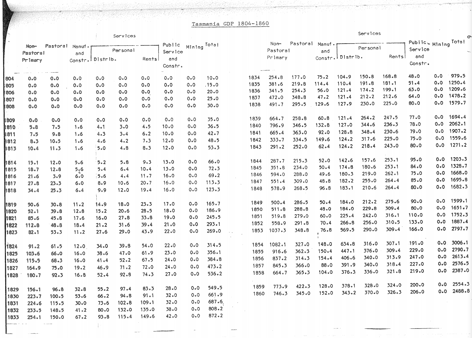
Historical and Colonial Census Data Archive (2019)
More specifically, let us examine the research of Peres-Cajías and Herranz-Loncán (2016) and their attempt to provide GDP per capita estimates for the Latin American country of Bolivia for 1890–1950. Their estimation strategy is prominent among researchers attempting to construct GDP estimates for periods in which crucial information is missing (e.g even Peres-Cajías and Herranz-Loncán [2016] refer to a long-line of scholars attempting to estimate the GDP for specific Countries in different periods of time).
Peres-Cajías and Herranz-Loncán’s (2016) GDP estimates are based on the production approach, with data from the Official National Accounts 1950 (refer to the table, below). To establish a consistent link between the series GDP and current GDP figures, all estimations begin at the value-added of each Bolivian economic sector in 1950 from the national accounts. These figures are then extrapolated backward with the assumption that real gross output for 1890–1950 evolved at the same pace. Finally, the sum of the resulting sectoral value-added series is the yearly estimation of the Bolivian GDP.
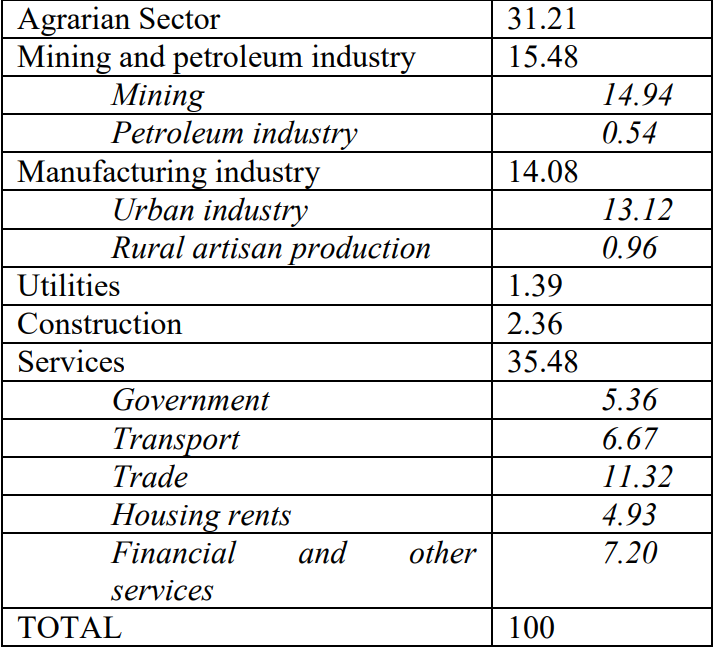
Sector percentages (in 1958 prices, the earliest available) as referenced in Peres-Cajías and Herranz-Loncán (2016)

Image 1.4 Angus Maddison (source: Maddison Project Database)
Angus Maddison
Several scholars have constructed and reconstructed national estimates for various premodern world economies using a variety of methods. However, the most cited and widely debated research about economic growth is by Angus Maddison. He describes himself as a chiffrephile – a lover of figures. His research improved upon and extended the work of Raymond Goldsmith. Maddison’s estimates were both restrictive and reasonable, assuming that per capita GDP was the same around the world before the Industrial Revolution.
Economic growth, like population growth, is a modern phenomenon. Before the Industrial Revolution, economic growth was nearly constant. Although, in the 16th century, there were minor income growths, productivity improvements only began after the Industrial Revolution. The consensus was that the majority of the populace hovered around a subsistence level. For instance, the highest observable income level in any society before 1000AD was at least twice the sustenance level in modern-day Italy, at the time, under the Roman Empire.
Since Maddison assumes that per capita GDP is the same across the world, he estimated the historical GDP of regions by multiplying the per capita GDP by each region’s population to estimate GDP. The methodology is logical. It is difficult to argue that Maddison was intentionally attempting to be dubious by using qualitative and unconventional approaches in his economic estimates because he updated his estimates to include new research findings and updated his methodology when there were more data.
Practices and Assumptions of Maddison's Estimates
Before 1820, estimates hardly existed. Therefore, Angus Maddison made strong assumptions. In several regions, these periods of insufficient data are often regarded as a “statistical dark age.” There now follows an explanation of some of these estimates:
Initially, Maddison (1995, 2001, 2007) used a single benchmark year for his extrapolations. This modern-day cross-country income comparison (Maddison selected 1990 for his first estimates, then changed to 2011 for subsequent estimates) used growth rates of GDP per capita from reconstructed national accounts to make comparisons for earlier years. This cross-country measure is designed to assess income levels across several countries. Often, this method was problematic because such comparisons were imbalanced – comparing “apples with oranges” and failing to consider effectively how certain goods mattered differently in different countries. The International Comparison Program (ICP) helped solve this problem.
Recent data and research on the ICP at the World Bank have used modern PPP to compare income levels in the 19th and early 20th centuries. Purchasing power parity was a concern because of the different consumption baskets; patterns across countries are difficult to reconcile because changing consumption patterns could distort estimates. Though some changes to the consumption patterns could easily be identified, data limitation increased the degree of uncertainty in these estimates. Therefore, early estimates of relative income levels differ significantly from standalone benchmark comparisons or independent estimates of relative income for those early periods.
In the most recent update of Maddison’s database, a multiple benchmark approach was implemented by the Maddison Database Project by choosing benchmarks for pre-1950 and post-1950 periods to make prices and incomes more comparable. Therefore, in the most recent estimates, real GDP per capita is in prices that are constant across countries.
For Asia and Africa, Maddison estimates GDP per capita was constant from 1500 to 1820. Moreover, GDP per capita grew at only 0.1% annually in Latin America and Eastern Europe, and at 0.2% in Western Europe. Perhaps, these numbers appear feasible because, for many African countries, there are simply no reliable population estimates until the 19th century. Maddison’s assumptions are attributed to Simon Kuznets’ estimates (1973). Maddison then extrapolates this further back by assuming that, before 1500, there was a subsistence-level GDP per capita, which is based on a Malthusian basic subsistence level. This level is pegged at $400 in 1990$.
Maddison estimates the GDP of every country by multiplying per capita levels by the population. With this, we learn that China was just barely above the subsistence level ($450 GDP per capita) in the first century. He also assumes that European per capita income levels were similar to those in China. This makes it reasonable to assume that per capita income in most of China was also similar. Evidence for this claim is based on an assessment of economic performance of the Roman Empire, which provided proof that the Roman levels were about two-fifths of Gregory King’s estimate of English income for 1688. Since West Asia and North Africa were part of the Roman Empire, Maddison also assumes that income was the same there. For the GDP for the Americas, Australasia, Southern Africa, Eastern Europe, and the former area of the USSR, subsistence levels are assumed ($400 GDP per capita). Thus, as Maddison explains, the measure is designed to account for the growth of GDP per capita over time. The measure is a combination of modern national accounts’ data and state-of-the-art reconstructions.
As difficult as it is to estimate the GDP per capita, it is just as difficult to estimate population. However, for countries such as Italy and China, there are census records as far back as the Roman Empire and Han Dynasty (206BC–220AD), respectively. In other regions, these estimates are made by using estimated cultivatable land.
How does Maddison’s data change over time? As stated previously, after Maddison’s death, some scholars have continued, “in the spirit of Maddison,” to publish an updated dataset of Maddison’s data. The project is called the Maddison Project Database. The database is updated by considering criticisms and including new findings from researchers. Estimates are adjusted as researchers investigate previously blank periods of historical GDP estimates. Therefore, it is common to see that new studies and their estimates are incorporated in the latest publications of the Maddison Database. Afterall, Maddison explained that his estimates were meant to challenge other researchers to produce their own findings and contribute.
It is important to note also the differences between the updates; the 2010 Maddison estimates miss some years between centuries. For instance, in 2010, there are estimates for 1000, 1500, 1600, 1700, and 1800. However, for the most recent updates, there are estimates for years in between, also. For example, in the 2018 update, there are estimates for 1AD, 730, 1000, 1150, and consistent yearly estimates from 1280 to 1500. These additions are a result of progress in the methods used by researchers regarding estimates for earlier years.
In generating his estimates, Angus Maddison used several studies, including his own research, to determine growth rate estimates. Regarding Scotland, for instance, Maddison assumes that the GDP was three-quarters of the level in England and Wales. For the period between 1500 and 1700, he assumes a higher growth rate because of the dynamism of Britain and most other European countries in terms of population growth, urbanization, and foreign trade.
More specifically, Maddison writes:
“For an appropriate picture for Western Europe as a whole, I made proxy estimates for Austria, Denmark, Finland, Norway, Sweden and Switzerland with the assumption that real GDP increased at 0.17 per cent annually between 1500 and1820. For Germany, a per capita growth rate of 0.14 per cent was assumed as there was a decline in Germany’s role in banking and Hanseatic trade, as well as the impact of the Thirty Years’ War When the proxy estimates are aggregated with the estimates for the five countries for which we have better evidence, we find average per capita growth for the 12 West European core countries of 0.15 per cent per year. This is significantly lower than Kuznets’ 0.2 per cent hypothesis…. I assume here that average per capita growth in ‘other’ Western Europe (Greece and 13 small countries were the same as the average for the 12 core countries).”
This method was used for other estimates across the globe. The method is not arbitrary because, when compared with the modern GDP numbers, the numbers appear appropriate, in the sense that there are no too large or small variations.
Conclusion: Problems and Shortcomings of Gross Domestic Product
There are arguments regarding the use of GDP to measure welfare or progress. Even Simon Kuznets, the father of modern GDP, acknowledged the problem of data availability as he submitted his findings to the US Senate in the 1930s. Therefore, using GDP as a measure of progress is often highly debatable by economists and economic historians alike.
While GDP may inform us about the economic tempo and temperature, it is often argued that it provides limited information on the distribution of wealth and ignores the negative cost of development regarding the sustainable development debate. Today, there are new methods to measure welfare, such as the Happiness Index and the Human Development Index (HDI). There have been recent efforts to backdate the Human Development Index using an interesting range of measures. However, this would require a separate article to do justice to the topic and its effectiveness. For now, it is sufficient to argue that there are correlations between GDP and other measures of welfare, such as the HDI, life expectancy, happiness, and wealth.
An interesting thought, in conclusion, concerns whether future generations will be able to measure our economy today effectively. Although there are global standards of reporting, how do we measure the digital economy? Some researchers have proposed methods such as asking people how much they would be willing to pay to use services like Google or WhatsApp, and then using this to measure the digital economy. Considering the importance of the digital economy, failing to measure it may mean significantly underestimating or overestimating the economy, which could affect the direction of future research.
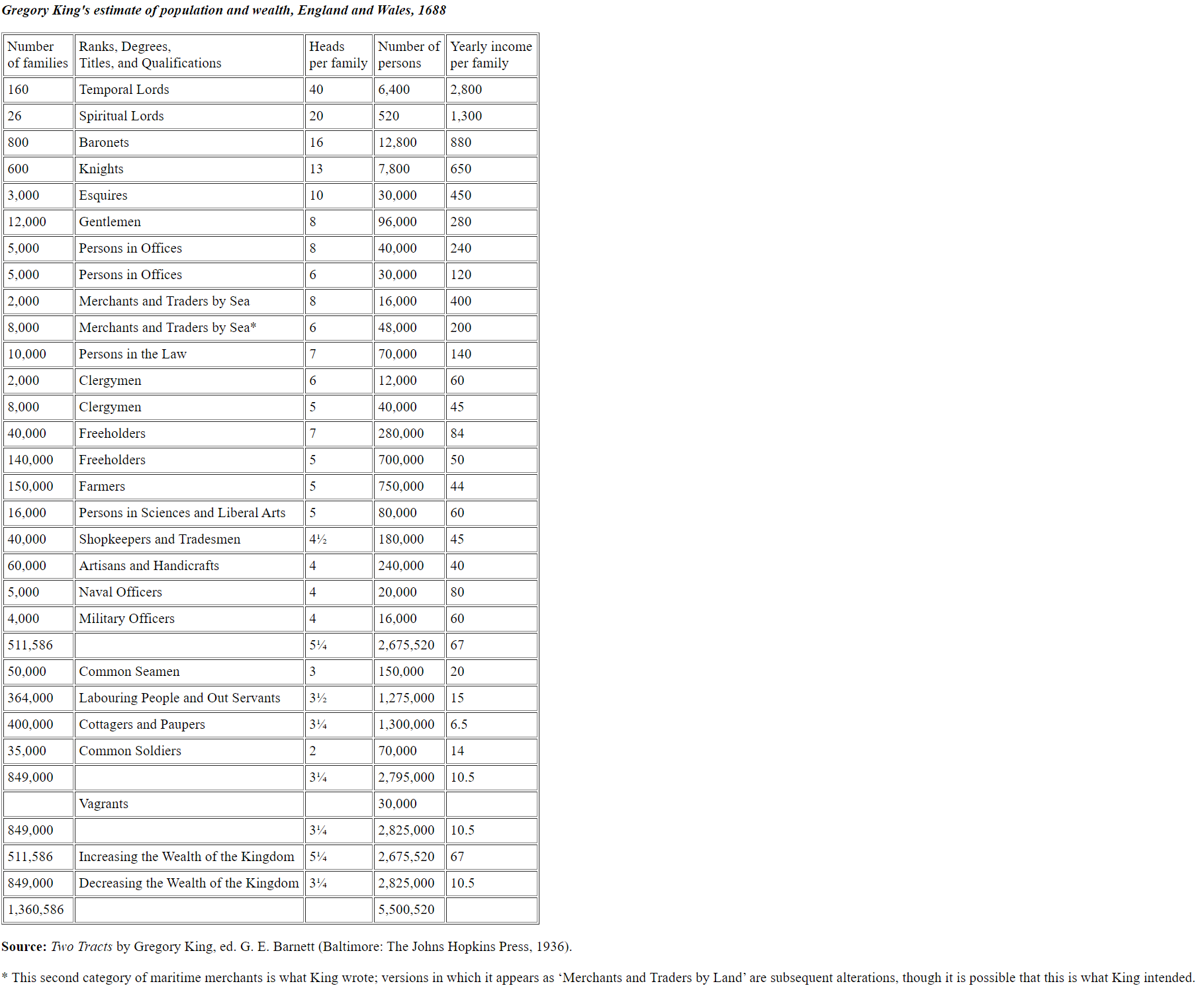
Image 1.5 Gregory King’s estimate of population and wealth, England and Wales, 1688. Source: (University of York)
References
Acemoglu, D. & Robinson, J., 2012. Why Nations Fail. US: Crown Business.
Allen, R. C., 2007. India in the great divergence. In: T. J. Hatton, K. H. O'Rouke & A. M. Taylor, eds. The new comparative economic history: essays in honor of Jeffrey G. Williamson. Massachutes: Cambridge, pp. 9-32.
Allen, R. C., 2013. Poverty lines in history, theory, and current international practice, UK: Oxford Press.
Allen, R. C. et al., 2011. Wages, prices, and living standards in China, 1738-1925: in comparison with Europe, Japan and India. Economic History Review, 64(1), p. 14.
Álvarez-Nogal,, C. & Prados de la Escosura, L., 2013. The Rise and Fall of Spain (1270-1850). Economic History Review, Volume 66, pp. 1-37.
Baten, J. & Blum, M., 2014. Human Height since 1820. In: J. L. van Zanden et al, ed. How was life? Global well-being since 1820. Paris: s.n., pp. 118-38.
Blaut, J., 2000. Eight Eurocentric Europeans. New York: Guilford Press.
Bolt, et al., 2018. Rebasing ‘Maddison’: new income comparisons and the shape of long-run economic development, Colombia: Colombia University Press.
Bolt, J. & van Zanden, J. L., 2014. The Maddison Project: collaborative research on historical national accounts. The Economic History Review, 67(3), pp. 627-651.
Broadberry, S., 2006. Market Services and the Productivity Race, 1850–2000. Cambridge: Cambridge University Press.
Broadberry, S. et al., 2015. British Economic Growth 1270-1870. Cambridge: : Cambridge University Press.
Broadberry, S. G. & Li, D. D., 2018. China, Europe, and the Great Divergence: A Study in Historical National Accounting. The Journal of Economic History, 79(2), pp. 470-560.
Broadberry, S. N. et al., 2014. British Economic Growth, 1270-1870. Cambridge: Cambridge University Press.
Butlin, N. G. & Sinclair, W. A., 1984. Australian Gross Domestic Product 1788-1860. Monash: Australian National University.
Chaney, E. & Hornbeck, R., 2015. Economic Dynamics in the Malthusian Era: Evidence from the 1609 Spanish Expulsion of the Moriscos. The Economic Journal, August, Volume 126, p. 1412.
Clark, G., 2007. A Farewell to alms: A brief Economic History of the world. Princeton: Princeton University Press.
Deaton, 2008. Income, Health, and Well-Being around the World: Evidence from the Gallup World Poll. Journal of Economic Perspectives, 22(2), pp. 53-72.
Diamond, J. & Robinson, J., 2010. Natural Experiments in History. Boston: Havard University Press.
Fourie, J. & Van Zanden, J. L., 2013. GDP in the Dutch Cape Colony: the Nationals Accounts of a Slave-Based Society. South African Journal of Economics, 81(4), pp. 467-490.
Goldsmith, R. W., 1984. An Estimate of the size and structure of the National Product of the Early Roman Empire. Review of Income and Wealth, 30(3), pp. 263-288.
Gommans, J., 2015. For the home and the body: Dutch and Indian ways of early modern consumption. In: M. Berg, F. Gottmann, H. Hodacs & C. Nierstrasz, eds. Goods from the east, 1600–1800: trading Eurasia. s.l.:s.n., pp. 331-49.
Kramp, P. L., 2020. Gross Domestic Product and Welfare. Monetary Review, pp. 95-99.
Lucassen, J. & Pim De Zwart, 2020. Poverty or Prosperity in northern India? New Evidence on real wages, 1590s-1870s by Pim De Zwart and Jan Lucassen. The Economic History Review, 73(3), pp. 644-667.
Maddison, A., 1995. Monitoring the World Economy 1820–1992. Paris: Organisation for Economic Cooperation and Development.
Maddison, A., 2001. The World Economy: a Millennial Perspective. Paris: Organisation for Economic Development.
Maddison, A., 2006. The World Economy: Historical Statistics. Paris: Organisation for Economic Development.
Maddison, A., 2006. The World Economy: Historical Statistics. Paris: Organisation for Economic Cooperation and Development .
Maddison, A., 2007a. Chinese Economic Performance in the Long Run. Second Edition ed. Paris: OECD.
Maddison, A., 2007. Contours of the World Economy, 1-2030 AD. Paris: Oxford University Press.
Palma, N., 2019. Historical Account Books as a Source for Quantitative History. Maddison-Project Working Paper WP-13, September.p. 4.
Patnaik, U. & Patnaik, P., 2016. A Theory of Imperialism. First Edition ed. New York: Columbia University Press.
Pomeranz, K., 2000. The Great Divergence: China, Europe, and the Making of the Modern World. Princeton: Princeton University Press.
- Peres-Cajías, José. (2014). Bolivian Public Finances, 1882-2010. The Challenge to Make Social Spending Sustainable. Revista de Historia Economica - Journal of Iberian and Latin American Economic History , Volume 32 , Issue 1 , March 2014 , pp. 77 – 117 DOI: https://doi.org/10.1017/S0212610914000019
- The Economist, 2013. What was the Great Divergence?, London: s.n.
The Economist, 2014. China's Back, Höchberg: Vogel Druck und Medienservice GmbH.
Utsa , P., 2018. Dispossession, Deprivation, and Development.. In: A. Banerjee & C. P. Chandrasekhar, eds. Essays for Utsa Patnaik. Colombia: Colombia University Press.
van Zanden, J. L. & van Leeuwen, B., 2012. Persistent but not Consistent: The Growth of National Income in Holland, 1347-1807. Explorations in Economic History, Volume 49, pp. 119-130.
- Voth, H.-J. (n.d.). Living standards and the urban environment. The Cambridge Economic History of Modern Britain, 268–294. doi:10.1017/chol9780521820363.011

Abdulrahman Tiamiyu
MA History & Economics Student